Houdini:
Organic Particles
Houdini is well known for complex fluid simulations using FLIP, but did you know that the POP solver has a POP Fluid node that uses the same techniques as FLIP but just a lot simpler and faster?
In this study we'll look at using that node to create microscopic fluids simulations that look like cells, or bacteria? Anyway, let's begin by creating a surface for our life to start from. In this verison we'll just use static points so the life has a simple source to grow from.
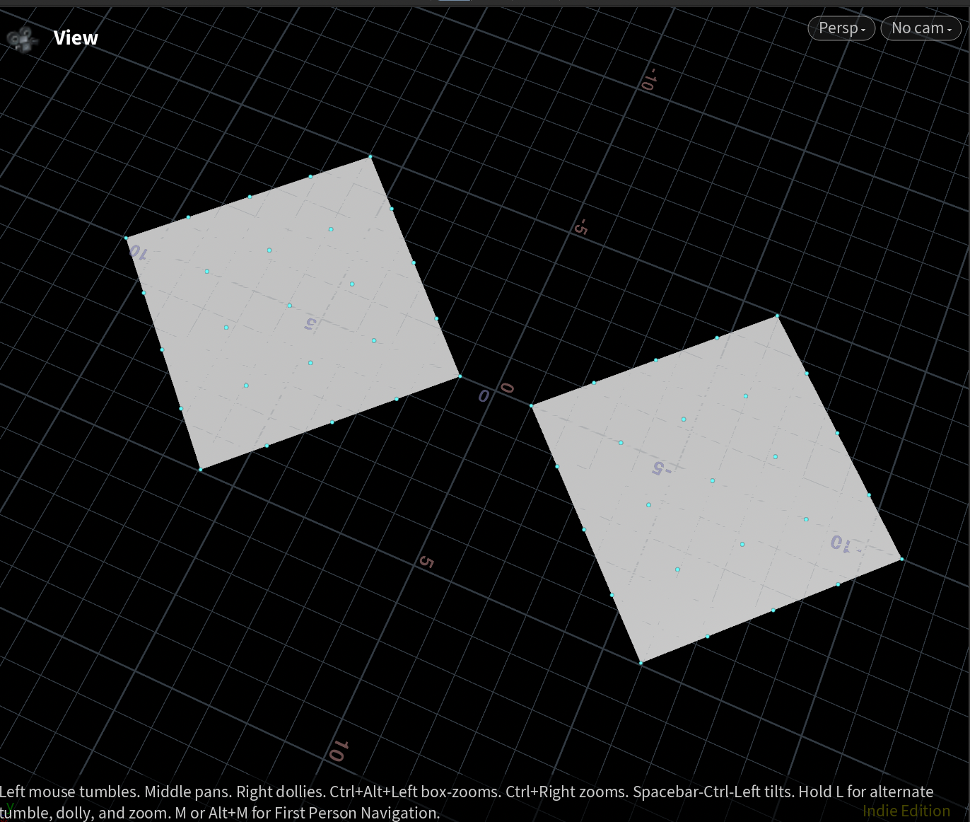
I used 2 flat planes with only a few divisions to start from, nice and geometric and clean.
Diving into pops, set the pop-source to "all points", this takes the input points every frame. When you press play nothing seems to happen. the points are being spawned but they are just placed right on top of each other.
Next is the POP Fluid node, still nothing seems to change but that's because the POP Fluid needs a little push, it needs the position to have just a tiny bit of distance between to work. So let's create some noise by adding a POP Wind node and increasing the amplitude in the Noise settings to somethign very low, 0.001.
Great, we have something happening. You can see the pop fluid node creating a distance between the particles and trying to create the shapes together in little blobs of liquid.
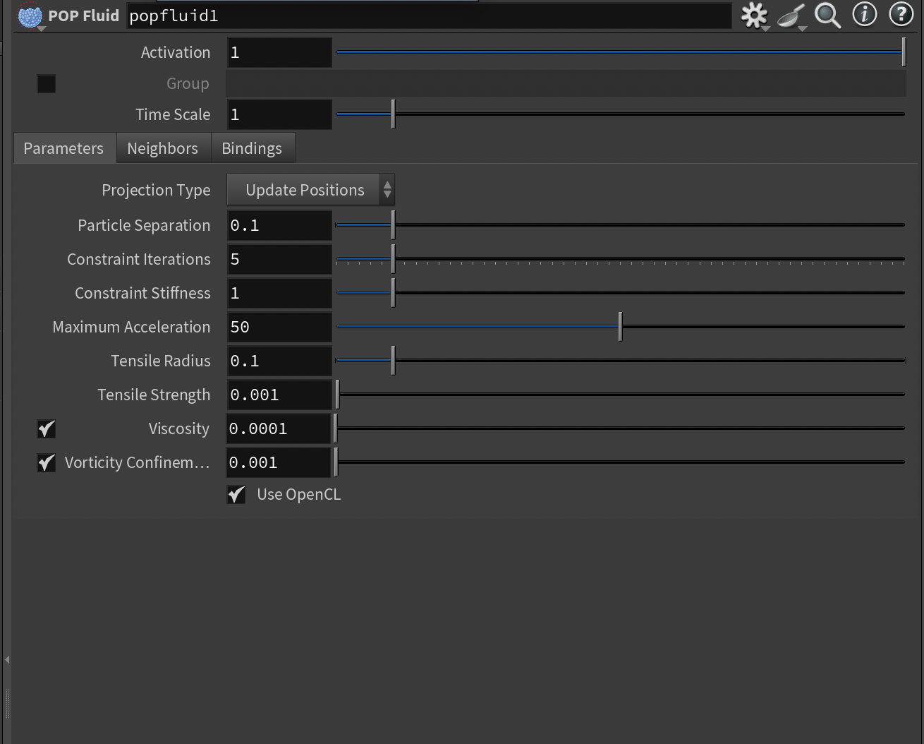
The POP Fluid node has a lot of settings, the ones we're most interested in are the constraint iterations and stiffness. Higher stiffness will create more even "blobs", but it does require more iterations, so it's a little slower to calculate.
Great, our system is creating cells, but what I wanted to try was to create that type of microscope cell effect, what that means is flattering the shapes. To do that we just make a tiny vex script in our solver.
Add a POP Wrangle and write:
@P.y = 0;
This flattens the fluid forcing it to find boundaries in only one axis. This creates an interesting effect where the borders of the fluid start to resemble a cell wall, play around with the settings to find out which effect you like the most.
When the expanding shapes find each other, the call walls merge into each other, creating a satisfying "merging" effect.
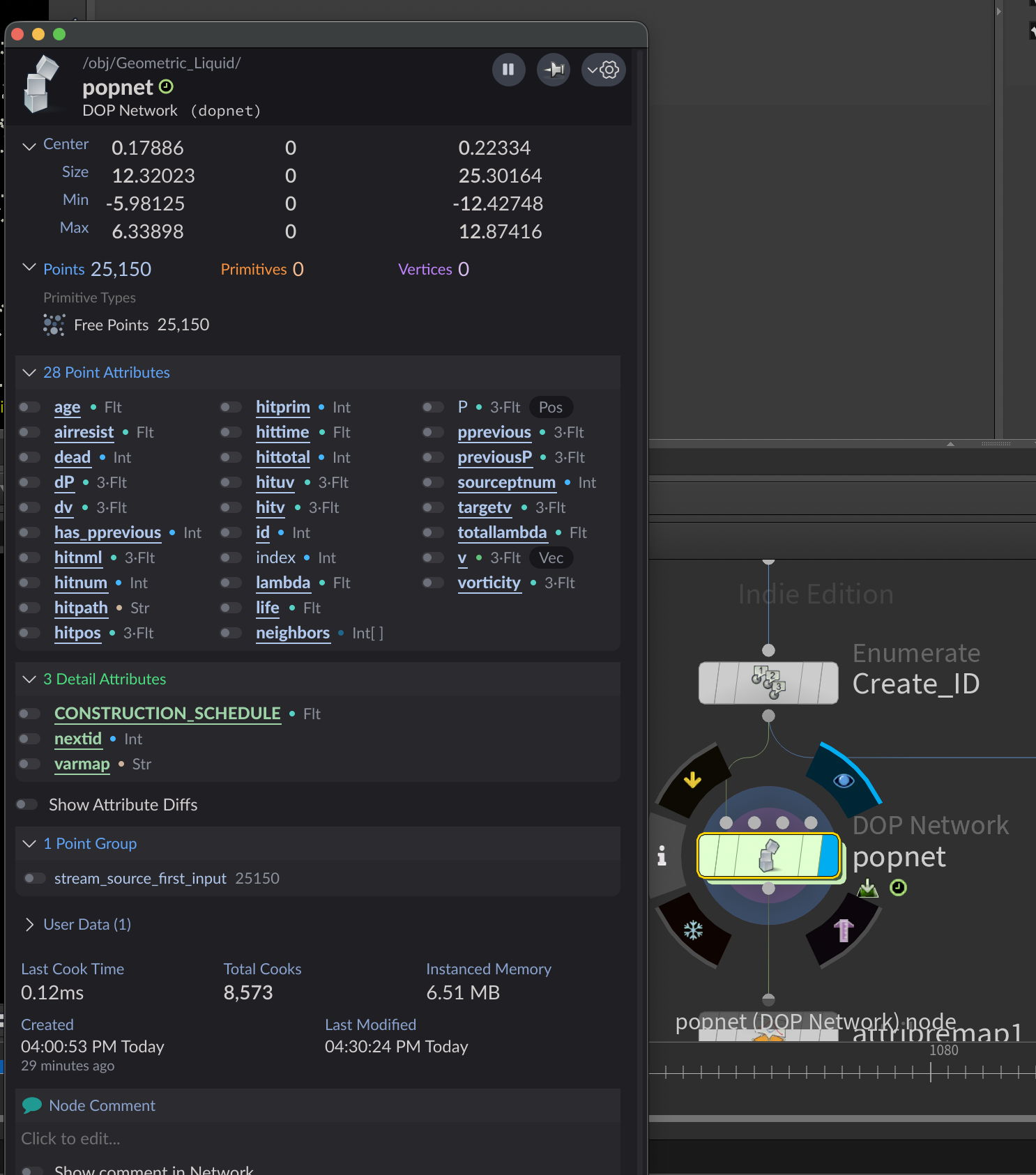
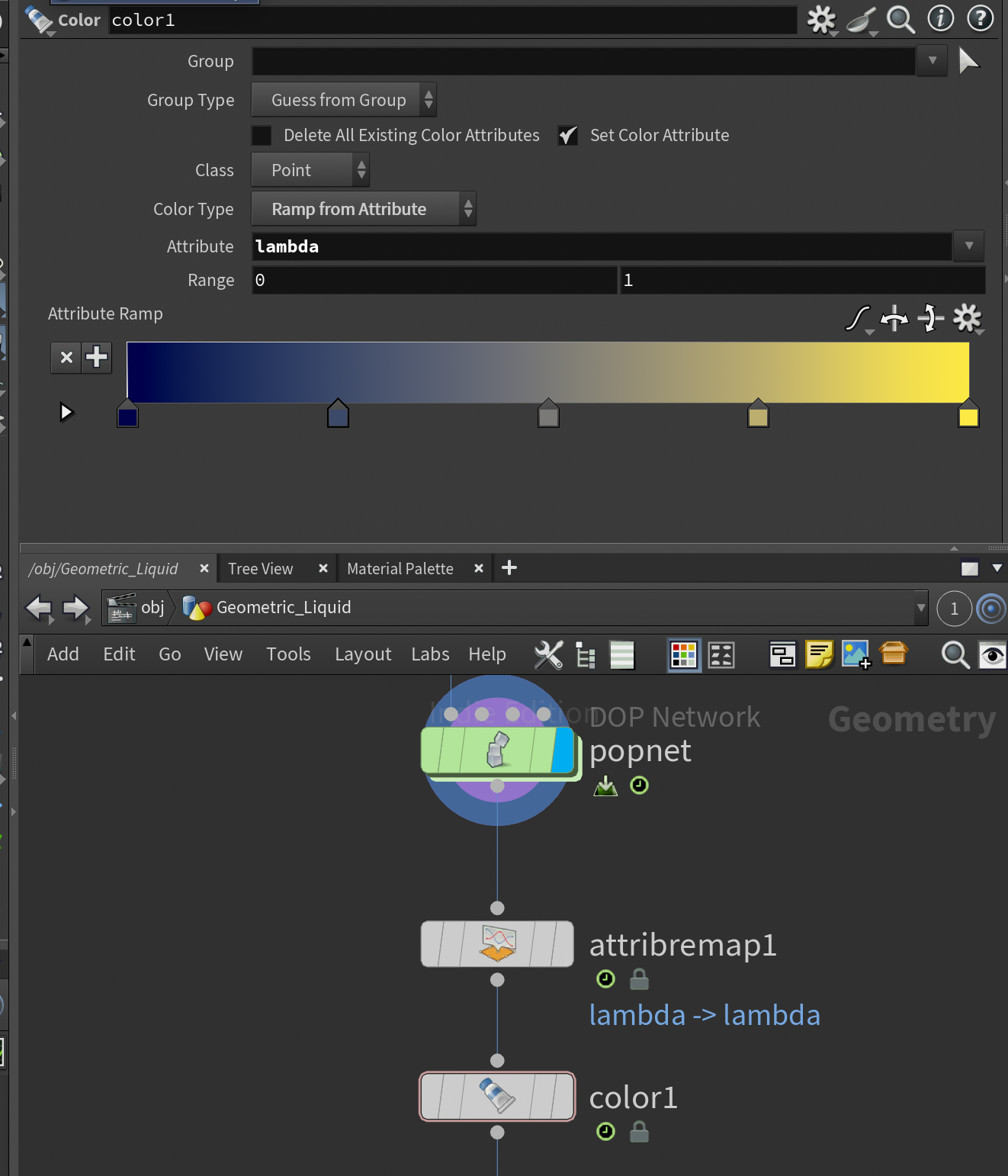
That's it for the particles. Let's jump up one level back to our shapes. You can see that the POP Fluid creates a lot of attributes. Some are more useful than others, but the one we're interested in is called the "lambda" or "totallambda", it's a bit complex but you can imagine it as a gradient from the "edge" of our fluid to the "center" of our fluid. In our flat fluid it visualises the cell wall quite well!
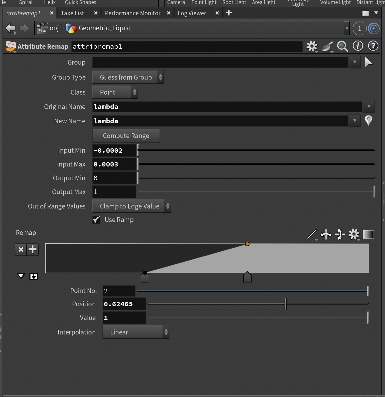
Let's remap the lambda by using an Attribute Remap node, then pressing "Compute Range", this should change the input and output ranges. Change the output range to 0 and 1 to create an easy to understand 0-1 gradient.
Then create a Color node and choose ramp-from attribute and choose our newly remapped "lambda" attribute. And choose a nice gradient. You might have to play around with the settings in the attribute remap, try something between -0.0001 and 0.0005, it's a pretty small number but you should be able to get a visualisation of our cell wall.
To add a bit more visual flair, we can use a Trail node to create trails, which makes things a bit more dynamic if you'd like. Use high trail length and low iteration settings for a better result.
And that's it! You can add a lot more nodes in our pop simulation, try a more intense noise or a pop-drag to control the movement more.
Let me know what you made, you're always welcome.